Application Specific Integrated Circuit (ASIC) Floorplan Automation - Part II

Written by Wooshik Myung on 07 Dec 2023

Reinforcement learning, take on the challenges of the industry! – ASIC semiconductor design (Floorplan) automation (Naver Deview 21 presentation video) )
Application Specific Integrated Circuit (ASIC) Floorplan Automation - Part I

Abstract

Introduction

The primary goal of this project is to leverage reinforcement learning to address the placement optimization problem within the floorplan, a crucial part of the Application Specific Integrated Circuit (ASIC) manufacturing process. This project’s core technical content is heavily influenced by the publication A graph placement methodology for fast chip design[1][2], which Google published in June 2020 and quickly gained recognition upon its inclusion in the Nature. Floorplan involves arranging blocks rather than individual transistors, making it one of the most time-intensive phases due to the intricate positioning required while taking into account connectivity with tens to millions of transistors. In this post, we aim to elucidate the process we underwent over approximately five months, from identifying the floorplan to executing the solution.

To provide context, let’s introduce some key terms and their definitions that will reappear throughout this text.

Macro: A memory component that is substantially larger than standard cell, frequently used in the floorplan process.
Standard Cell: A small-sized logic gate, such as NAND, NOR, or XOR, housing tens to millions of components.
Net: The wiring that connects the macro and standard cells.
Netlist: A list of nets.

Is this a Real Problem?

The floorplan process is usually performed manually, involving the placement of hundreds of macros within a two-dimensional continuous space known as the chip canvas. This task is inherently challenging due to the vast search space and the intricate connections that must be considered. After macro placement, the subsequent design process can be assessed using a specific Electronic Design Automation (EDA) tool. If the evaluation result is poor, the macro placement process must be repeated. The variability in results, combined with the differing levels of expertise among technicians, results in a substantial variance in the time required. Even for skilled experts, this process can extend for days or weeks. In collaboration with professionals in this field, we have identified the following issues in the floorplan.

Manually placing macros requires a significant amount of time to evaluate the results, necessitating numerous iterations with the EDA tool.
With varying skill levels among technicians and experts, the quality of outcomes and the time required vary considerably.

This post focuses on the technical aspects of problem formulation and its solution. (For a more detailed description of the research background and significance, please refer to ASIC-Chip-Placement Part I.)

How to solve?

Classical approaches like Simulated Annealing[3] and Genetic Algorithm[4], when applied in placement optimization*, have demonstrated strong performance. However, they share a common drawback – when faced with a new problem, even within the same domain, they necessitate starting the optimization process from scratch. Overcoming this limitation requires a concept known as generalization, where a trained model can find solutions above a specific threshold without the need for additional training on newly defined problems. Multiple studies[8][9] have demonstrated that reinforcement learning, when coupled with artificial neural networks, possesses a remarkable level of generalization. This capacity empowers it to identify suitable placements for netlists of diverse structures and sizes, often without the need for extensive additional training (e.g., it can learn the optimized placements of netlists containing 5 and 10 components and apply that knowledge effectively to manage netlists comprising 20 components). Our primary focus has been on harnessing this capability, and we have employed reinforcement learning as the core algorithm. In this article, we’ll delve into a single netlist floorplan learning procedure that employs reinforcement learning, guiding us towards our end goal: achieving generalization.

* Placement optimization: The problem of optimizing the objective function through the physical location of the target.

What is reinforcement learning?

Reinforcement learning is an algorithm in which an agent learns higher-rewarding actions through trial and error by interacting with the environment. For each action taken by the agent, the environment provides feedback in the form of states and rewards. Based on this feedback, the agent decides on the next action to take. Reinforcement learning is rooted in the principles of the Markov Decision Process[5] (MDP) and is widely used to solve problems that require decision-making.

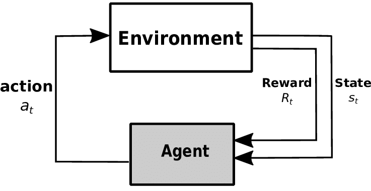
markov decision process — [Figure ] - Markov Decision Process

By the end of the learning process, the agent acquires the behaviors that maximize the expected reward value across all sampled episodes*. The specific learning patterns that emerge from reinforcement learning depend on how we define its core components: the agent, the observation, the action, and the reward. In the following section, we’ll discuss how we defined the environment and the agent.

* Episode: The sequence in which the agent performs a series of actions and receives rewards (state, action, rewards), after which the environment is reset to its initial state.

Technical Overview

We will first discuss the broad flow of the environment and how the neural network model works, followed by a detailed definition of each part of reinforcement learning.

Environment

Agents learn by interacting with the primary components of the environment, namely state, action, and reward. To effectively train an agent, it’s crucial to accurately define each of these components. The role that each part of the environment should play in optimization are as follows:

State: Must contain the information needed to decision-making when determining action
Action: A series of actions that allow for a better floorplan
Reward: Chip design quality

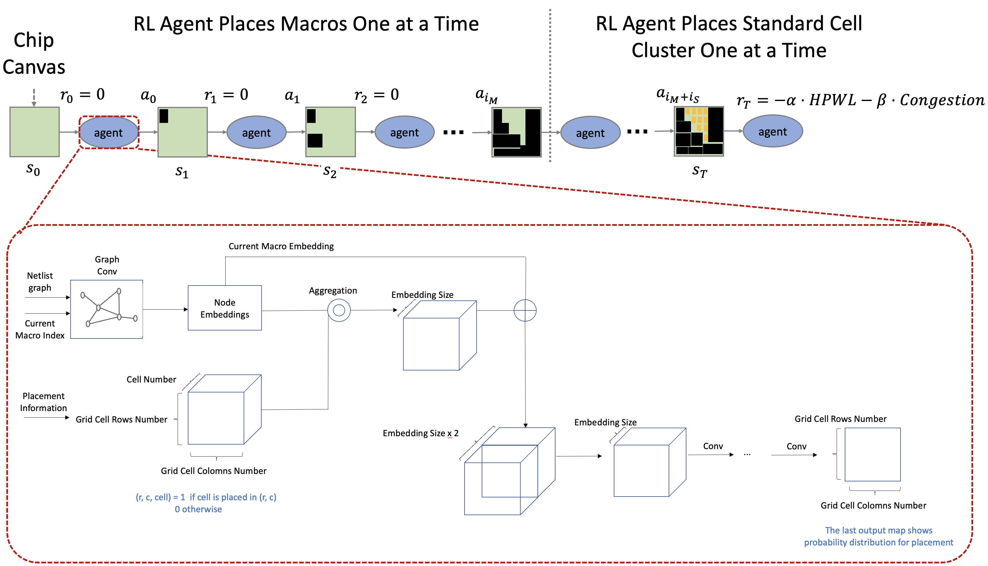
Our proposed environment will proceed in the following order:

Place each component one at a time, starting with an empty chip canvas in its initial state.
For all placements except the last, zero reward is assigned.
After repeating steps 1 and 2, the reward is calculated when all components are placed.
Repeat steps 1 to 3 to progress learning.

Let’s begin by discussing the model design before we define state, action, and reward.

Neural Network Architecture

role op model — [Figure ] - NN architecture

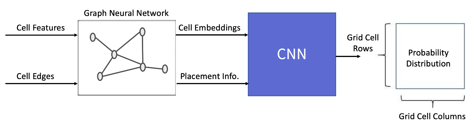
The neural network architecture is responsible for calculating the probability distribution of available actions based on input from the observations. In this project, we require information about both the components that have already been placed and those that will be placed in the future, considering their physical properties and connectivity. To do so, we’ve developed a model that combines Graph Neural Network (GNN) and Convolutional Neural Network (CNN). The roles of these networks are as follows:

GNN: We chose this approach to effectively embed the netlist’s information in the form of a graph.
CNN: The CNN structure was adopted to gather local information on the deployed components.

A detailed description of each model structure will be given in the chapter on Model Description.

RL Environment

State Representation

The state provides information about the current state of the environment. This state should convey information that helps the agent in determining the appropriate course of action. The information required by the agent to select the next action is described as follows, considering the placement of the chip design experts and taking into account the connectivity and physical properties of the components:

Connections between the components
Physical information of each component (e.g., width, height, is_macro, n_pins, …, etc.)
Information on the components to be placed this time
Information about the components placed so far

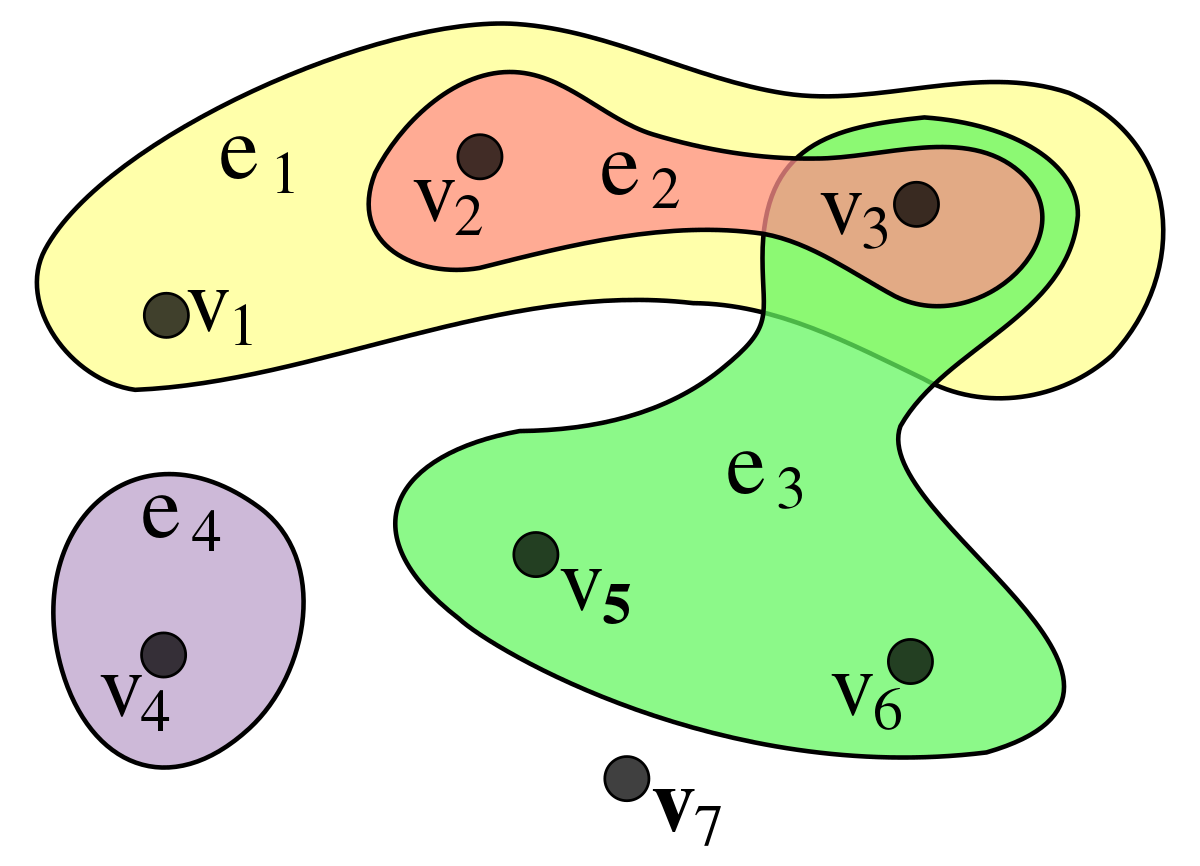
The physical features of each component can be specified as node features, and the connections between each component take the form of a hypergraph*, as illustrated below.

* Hypergraph: A graph structure in which two or more Vertices are connected to a single Edge.

Compared to the installation of hundreds of macros, placing tens to millions of standard cells is considered more challenging. Components are clustered to simplify the process of placing standard cells. Clustering reduces the complexity of the problem by reducing the number of targets that need to be placed. To minimize information loss when converting a hypergraph to a oridinary graph*, the hMETIS[6] algorithm, a hypergraph clustering algorithm, is employed. The components belonging to one cluster are aggregated and treated as one separate component in the subsequent placement procedure.

* Ordinary Graph: A graph in which two vertices are connected by a single edge.

Action Representation

The action plays a role in determining where to place a component based on state information (physical properties of the components, current placement, etc.). To optimize the agent’s reward, sufficient exploration is necessary. It’s crucial to define the appropriate size of the exploration space to make the exploration more efficient. With these considerations, we have defined the chip canvas as a discrete space on a two-dimensional grid within continuous space. When the agent selects a specific grid cell* from the probability distribution obtained by the neural network, the center of the component to be placed is positioned at the center of the corresponding grid cell.

* Grid cell: A unit corresponding to one space in a 2-dimensional grid

The benefit of defining the canvas as a grid is that it simplifies the provision of an approximated metric for analyzing placement outcomes while also saving space. Please refer to the APPENDIX for information on how to overcome the challenges listed below, which should be considered when defining the grid.

A.1. Grid Cell Size Decision
A.2. Invalid Action Masking

Reward Representation

The agent’s reward is an essential aspect in determining the usefulness of its actions. ASIC floorplan is typically measured with dedicated EDA tools like ICC2. Additional design processes performed by the EDA tool to evaluate the placement outcome following the floorplan typically take several hours. Considering the slow calculation speed, it is fairly impractical to use the tool’s outputs to define a reward because reinforcement learning requires a large number of samples. Therefore, to collect more samples in the same amount of time, it is necessary to design a function that approximates the quality of the placement results in a short time.

To accurately estimate the quality of the placement results, one must first understand what constitutes a good placement. There are typically used criteria: PPA (Performance, Power, Area). The effects associated with each item are as follows:

Performance - High clock frequency (Hz)
Power - Low power consumption
Area - Small chip canvas

All three of the aforementioned factors must be taken into account if the approximation function is to be used as the agent’s reward function. At first glance, it may seem that placing the components close together will minimize the data transmission path, resulting in increased power, performance, and a smaller area. However, in chip canvas, there are routing resources where the components will be placed. In other words, a routing path is required to send and receive data across components, but the available routing resources are limited. As a result, if the components are arbitrarily positioned close together, and the number of routing paths available in the unit area exceeds the number of routing resources available, the signal should be detoured to the other side, as illustrated in the diagram below.

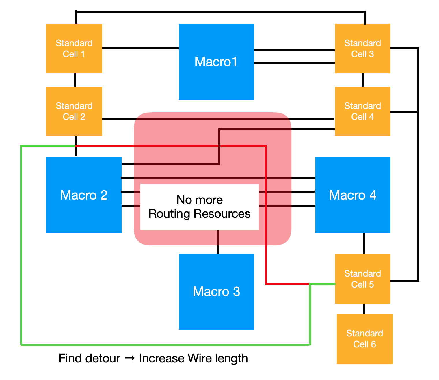
routing detour — [Figure ] - Routing Detour

The red line in the diagram above represents the shortest routing path for macro 2 and standard cell 5. However, due to the high density of routing paths in the red area, the actual signal transmission will be directed along the green line. Consequently, our objectives can be defined as follows:

'The distance between the components (wire length) should be kept as short as possible, while avoiding the congestion of too many routing paths in one location!'

In light of these objectives, the placement optimization problem becomes a multi-objective optimization problem, where component placements should be as close as possible, but not too close. The reward function designed to achieve this goal is as follows.

\[R_{p,g}=-\alpha \cdot WireLength(p,g) - \beta \cdot Congestion(p,g) \qquad \text{S.t. } \text{density*}(p,g) \leq \text{max}_\text{density}\]

* Density: Density of components placed in a unit area

Congestion aims to prevent an overload of routing paths in a single location, while wire length helps keep components close together. Below are the steps for calculating and applying each component.

Wire Length

To simplify the calculation process, the Half-Perimeter Wire Length (HPWL), an approximation of wire length, is used. By drawing a bounding box around each net’s components, we can estimate the wire length by calculating half of the total perimeter for all nets. HPWL is a widely used model for wire length estimation, as it is relatively simple to compute and provides an accurate length approximation, using an orthogonal steiner tree* for nets with 2 or 3 pins. The formal formula is as follows.

* Orthogonal Steiner Tree: One of the most commonly used methods for calculating the wire length of components is the Steiner Tree, which forms a right angle between Edges.

\[\begin{aligned} HPWL(i) = (\max_{b\in i}\{x_b\} - \min_{b\in i}\{x_b\} + 1) \\ + (\max_{b\in i}\{y_b\} - \min_{b\in i}\{y_b\} + 1) \end{aligned}\]

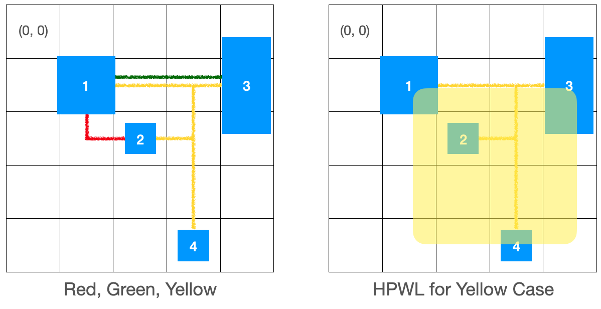
hpwl calculation — [Figure ] - HPWL calculation

If the figure on the left shows a wire with different colors of the routing path, HPWL is calculated as follows.

\[HPWL(Red)=(2 - 1 + 1) + (2 - 1 + 1) = 4 \\ HPWL(Green)=(4 - 1 + 1) + (1 - 1 + 1) = 5 \\ HPWL(Yellow)=(3 - 1 + 1) + (4 - 1 + 1) = 7\]

The approximation of the total wire length is 4 + 5 + 7 = 16. This formula is used to calculate the wire length of the nets.

Example Code

def calculate_hpwl(net: Net) -> float:
  """Calculate HPWL given Net."""
  min_row, min_col, max_row, max_col = get_boundary_coordinate_of_net(net)
  hpwl = (max_row - min_row + 1.0) + (max_col - min_col + 1.0)
  return hpwl

Congestion

Congestion is used to prevent routing paths from converging in a single location. It’s a metric that can only be precisely measured with specialized equipment, and it was a critical consideration during the environment design process. Congestion is characterized by the routing resources (supply) available in a given area and the net’s routing path (demand) in that area [7]. Both horizontal and vertical routing resources are taken into account separately.

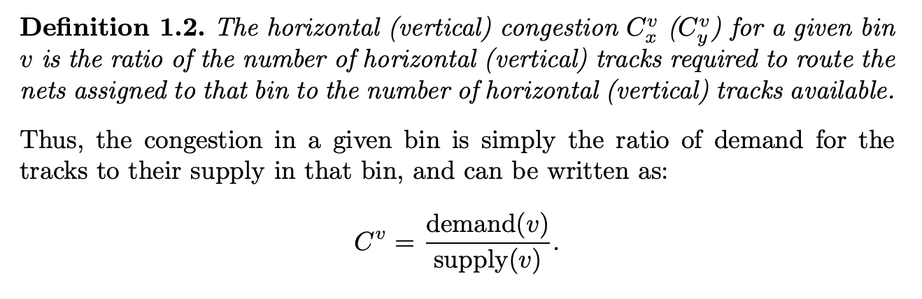
[Figure ] - Congestion[7]

Given the data we have, it’s not possible to directly measure supply. As a result, it is assumed that supply remains constant. According to this theory, congestion is primarily determined by demand. Taking this into account, we use the demand estimate calculated below as the congestion.

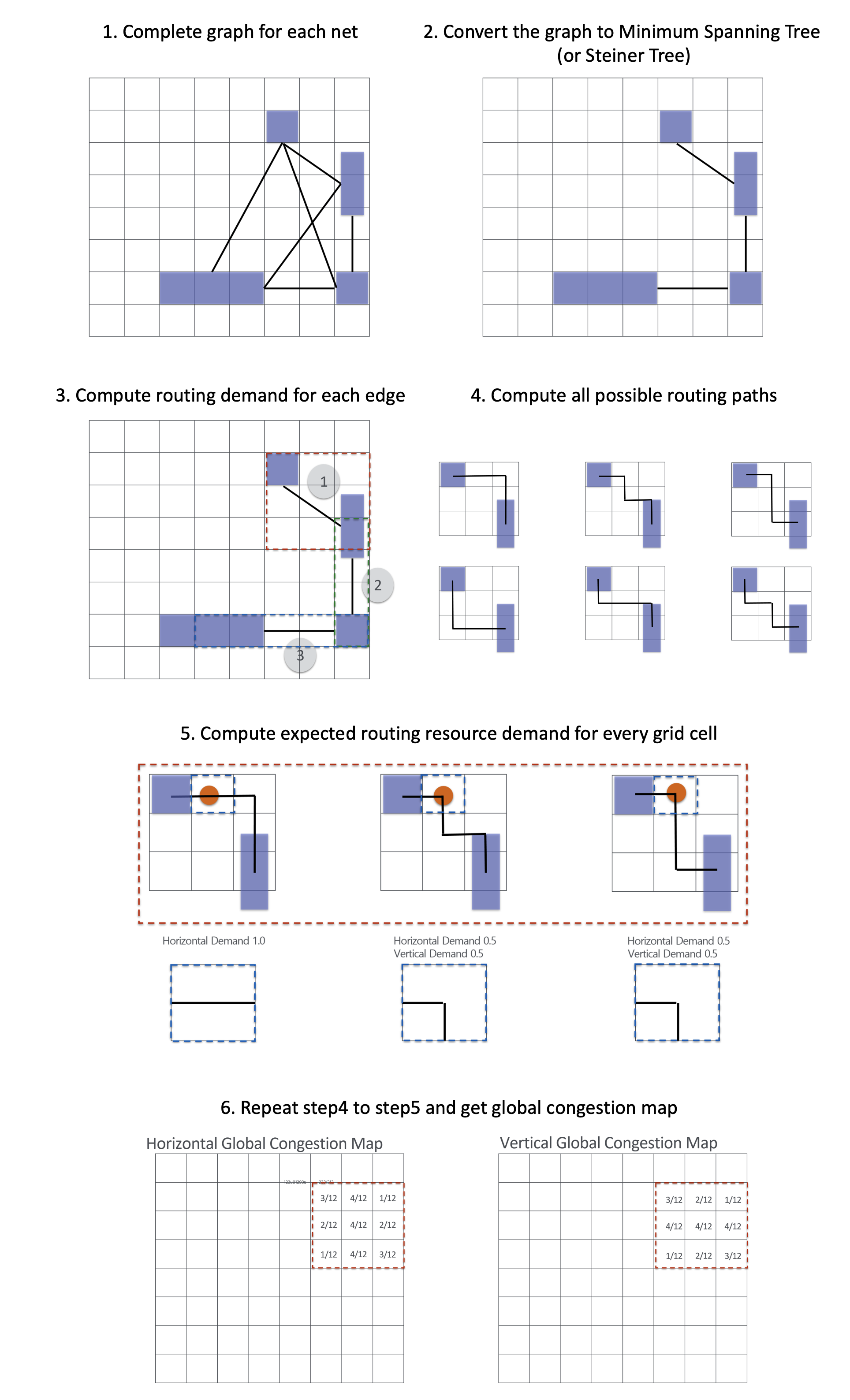
congestion calculation flow — [Figure ] - Congestion calculation process

Example Code

def accumulate_local_congestion(
  global_congestion_map: np.ndarry,
  net: Net
) -> None:
  """Accumulate local congestions into the global congestion map."""
  # get edges through MST or Steiner Tree
  edges = get_edges(net)

  for edge in edges:
    # Calculate all path number to source / target for all grid cells.
    paths = get_paths(two_pnt_net)
    # Calculate partial congestion map horizontally and vertically
    congestion_maps = get_congestion_map(paths)
  global_congestion_map += congestion_maps

The APPENDIX below summarizes the key considerations for creating reward functions.

B.1. Normalization & Reward Coefficient
B.2. Invalid Episode Handling
B.3. Convolution Filter

Model Description

To determine action, the model collects observations from the environment to calculate probability distribution. As highlighted in the state representation section, understanding the connection structure of the netlist and the current placement is crucial for making informed decisions. To achieve this, we have developed a two-stage model that combines GNN and CNN model. The GNN is responsible for embedding the netlist data, while the CNN calculates the probability distribution for actions based on the previously embedded data and the current placement. In most GNN models, the input data is defined as an ordinary graph. Therefore, we’ve implemented a preprocessing step to transform the netlist from its hypergraph form into an ordinary graph, allowing us to effectively use general-purpose GNN models. Below you’ll find a detailed description of the 2-stage model, including the preprocessing procedure.

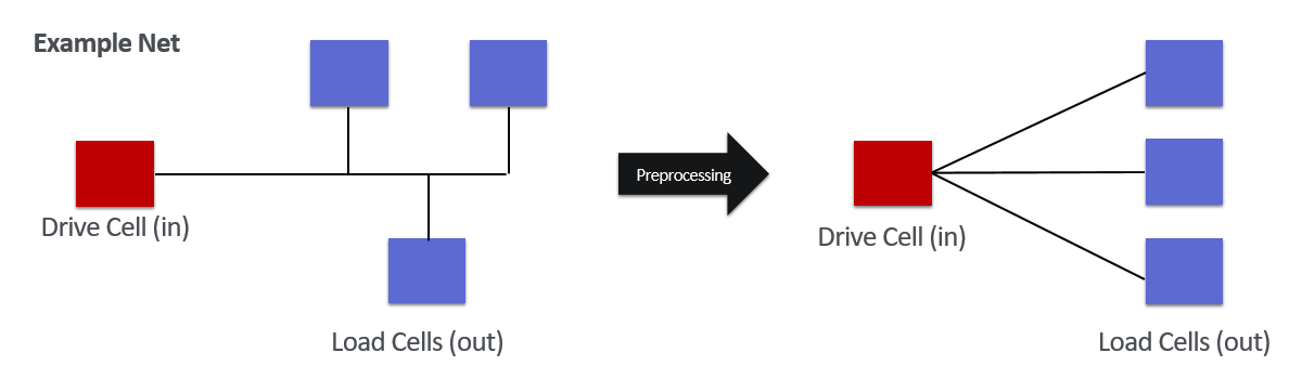
Hypergraph to Ordinary Graph

To make it easier to use and compare general-purpose GNN models that use ordinary graph, a net of hypergraph type is converted to ordinary graph type. During this process, the loss of connection information is inevitable. To minimize this loss, it is necessary to first comprehend the characteristics of the cells connected to the net. A hypergraph structure net consists of one drive cell and several load cells. The drive cell receives data and transmits it to the load cells. With these characteristics in mind, processing is performed in which the net in hypergraph form is turned into an ordinary graph form, with load cells connected to drive cells.

Graph Features Embedding

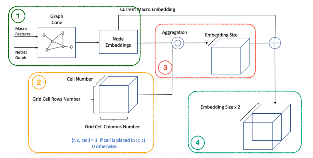
Graph Embedding — [Figure ] - Graph feature embedding

GNN was used to embed netlist information in the form of a graph. The following detailed steps outline the process of performing graph feature embedding:

Input macro features and netlist graph into GNN to extract node embeddings.
Display the placement of each component on the placement map (set the cell index value of each row and col to 1, otherwise 0).
Aggregate node embeddings based on the placement map information.
Concatenate the macro embedding by broadcasting it into the channel of the results obtained in Step 3.

In essence, each grid cell contains aggregated embedding of previously placed components (current placement + netlist connection information) as well as macro embedding for newly placed components (current placement information). The advantage of employing 3D embedding information lies in its ability to efficiently capture local information based on location using CNN, which, in turn, provides information for determining the appropriate placement area.

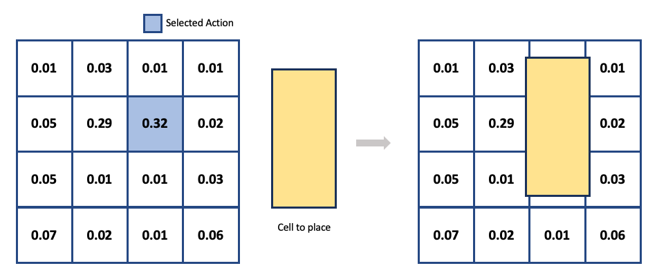
Action Decision

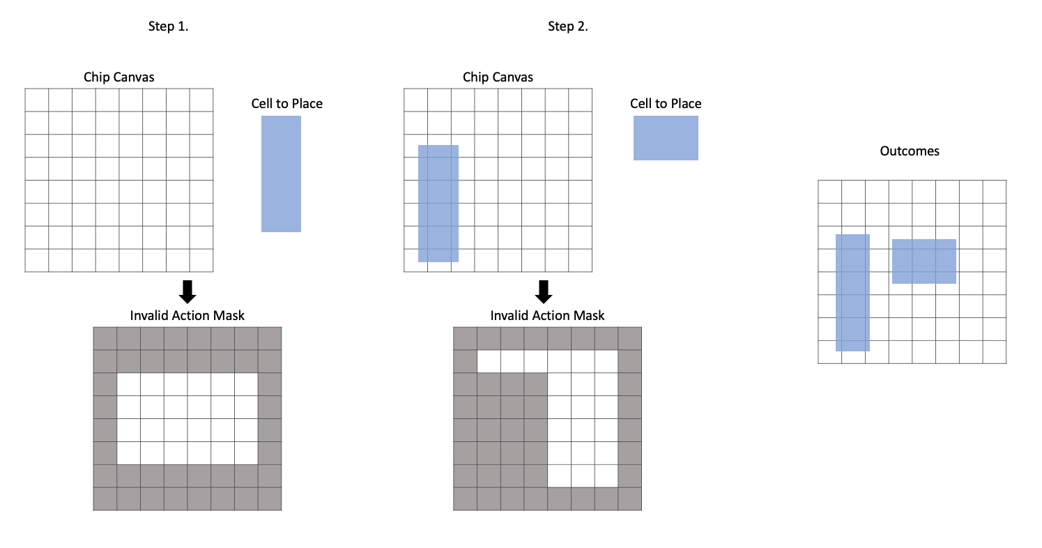
The information from graph feature embedding is interpreted as an image, and the probability distribution for the next component is calculated. Invalid Action Masking* is applied to the results from the final layer, and the component’s position is computed based on these values. This procedure is illustrated in the figure below.

* Invalid Action Masking: The task of determining where components can be placed, taking into account the conditions in which they are placed. (See APPENDIX A.2).

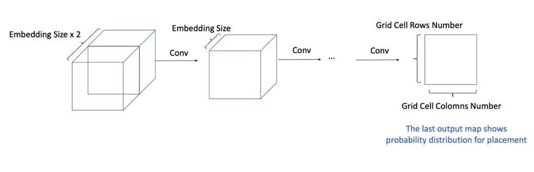
policy network — [Figure ] - Action Decision

Graph feature embedding is used in CNN to gradually reduce the number of channels to one. By altering the model’s depth or the size of the filter, the entire area of the chip canvas can be observed as the receptive field grows, and the input channel gradually decreases. The output of the final layer represents the probability distribution for the placement of the current component. The agent determines its actions based on this probability distribution.

Experiment Setup & Details

Dataset

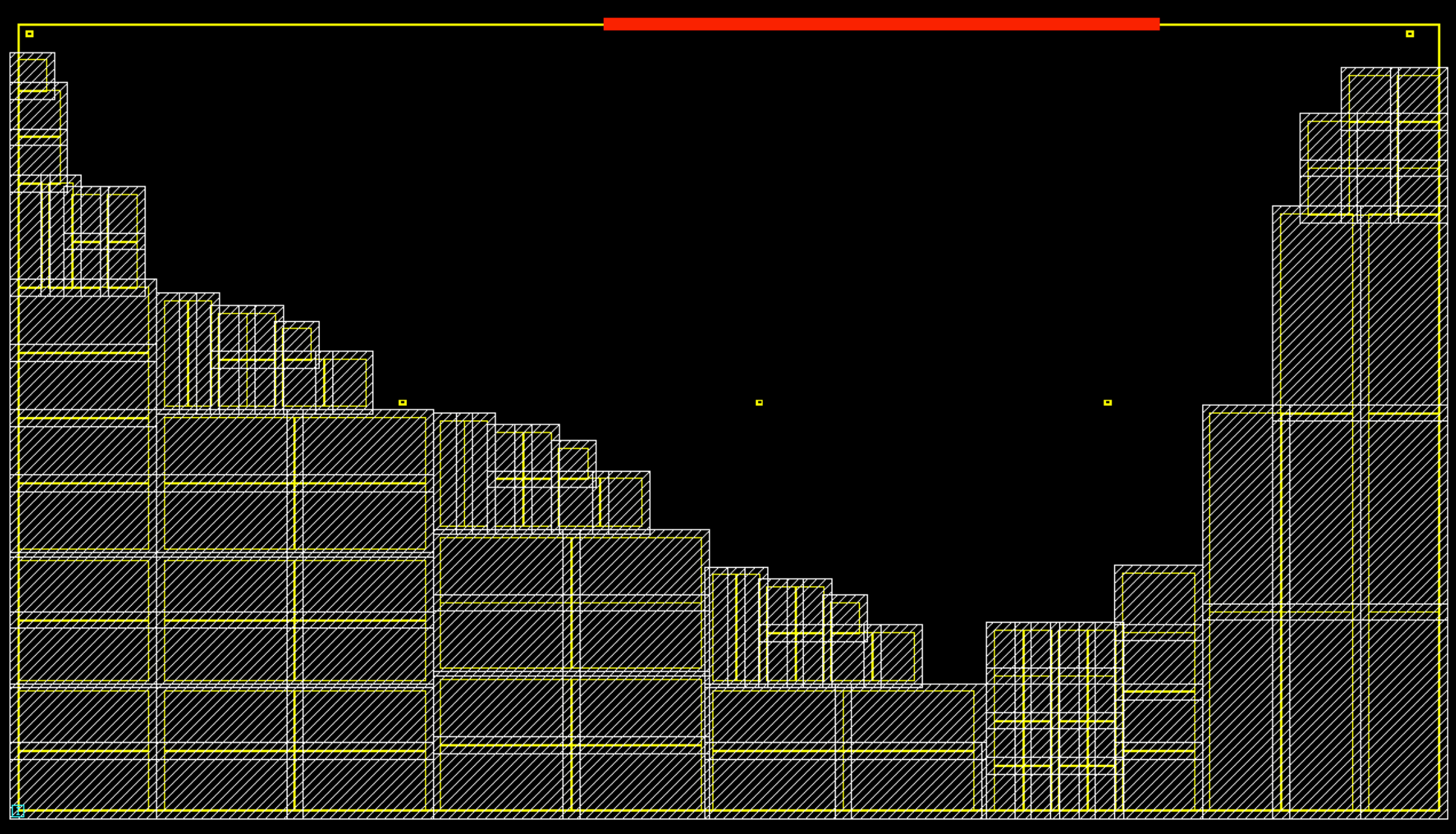
The following netlist was used to assess the effectiveness of reinforcement learning. Detailed specifications are provided in the table below (the placement in the figure is the result of macro auto placement of ICC2).

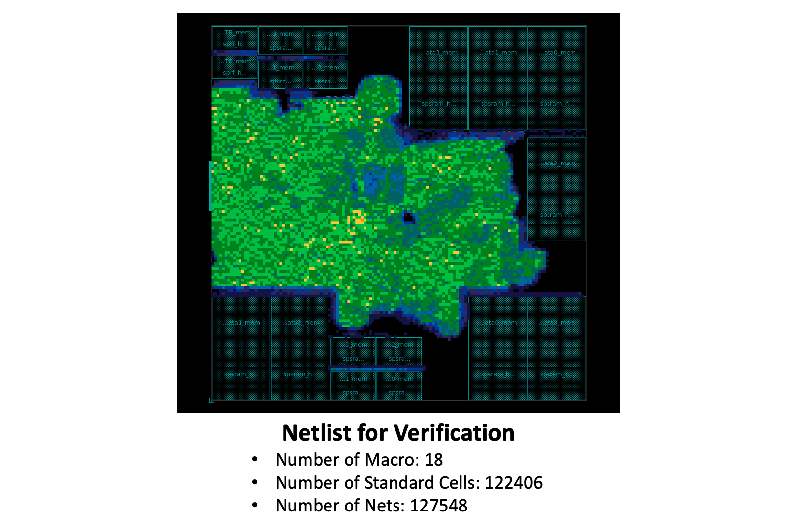
The corresponding netlist is made up of 18 macros and approximately 120,000 standard cells. The tests described below were conducted after compressing the standard cells into 50 clusters. To perform graph feature embedding, the Graph Convolutional Network (GCN) model was employed.

Evaluations

Two heuristics can be applied to reduce the complexity of the experiment.

Single Cluster

The primary objective of reinforcement learning is to identify the optimal placement of macros given the intricate connections within the netlist. We minimized the reliance on standard cells, and as a heuristic, made approximate predictions for standard cell positions. By grouping all standard cells into a single cluster and placing them together, we reduced the number of steps in each episode and simplified the link to macros, thus reducing the complexity of the learning process.

Bounding Box

In general, standard cells feature a high connection density. According to the results of actual chip placement experts, the macro is typically positioned on the outside of the chip canvas and the standard cell is located at the core for most component placement problems. This technique involves different layout sections for Macro and standard cell. By specifying the bounding box at the beginning of the learning process, we can restrict the search space by not inserting a macro within the defined region, thereby making the learning process more manageable.

Scenarios

We designed an experiment with the following scenario to test the effectiveness of reinforcement learning while gradually increasing the learning complexity.

Bouding Box + Single Cluster
Bouding Box
Vanilla RL w/o Heuristics

After applying both heuristics and then removing them one by one, a new batch is discovered using reinforcement learning without the use of a separate heuristic.

Scenario1: Bounding Box + Single Cluster

The first experiment was to use the single cluster and bounding box, which has the lowest complexity of the scenarios.

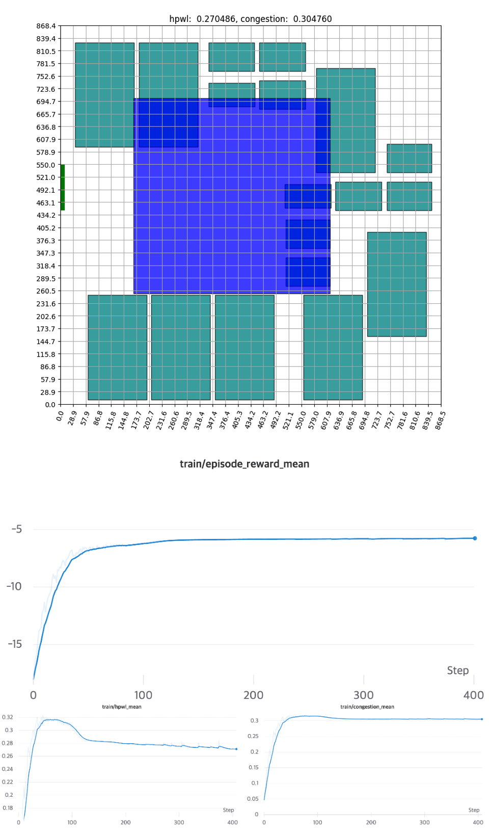
placment and training curve — [Figure ] - Results of placement and learning curve using single cluster and bounding box

As more of the macro’s area is assigned to the edge, the likelihood of not finding a placement in the early stage (Invalid Episode*) grows. Naturally, the initial HPWL and congestion average values are designed to be extremely low. As learning develops, it eventually begins to establish a stable configuration and converges, taking approximately 150 Epochs. The experiment demonstrates that the agent in reinforcement learning performs adequately at low complexity. 

* Invalid Episode: If all the possible areas disappear before all components are placed, HPWL and congestion are calculated as 0, and the reward is given as −α−β−α−β. (See APPENDIX B.2).

Scenario2: Bounding Box

In the second experiment, we increased the number of clusters in the first scenario to train at a higher complexity. By only using the bounding box, the compensation can become more sensitive to changes in the position of macros and clusters. The following are the training outcomes.

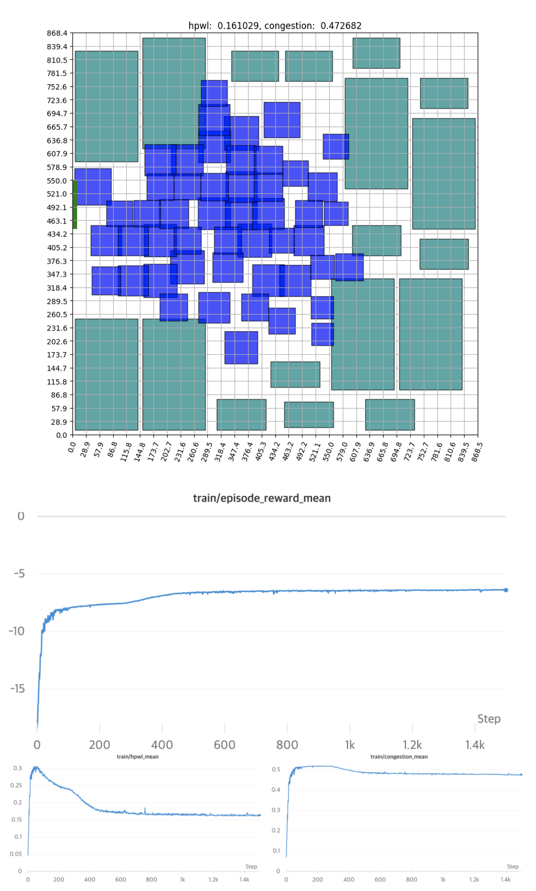
Due to the influence of the bounding box, several invalid episodes occur in this scenario as well. We can see, however, that this likewise resolves swiftly and converges around 500 Epochs.

Scenario3: Vanilla RL

In the previous scenario, we trained solely through reinforcement learning, without the use of additional heuristics.

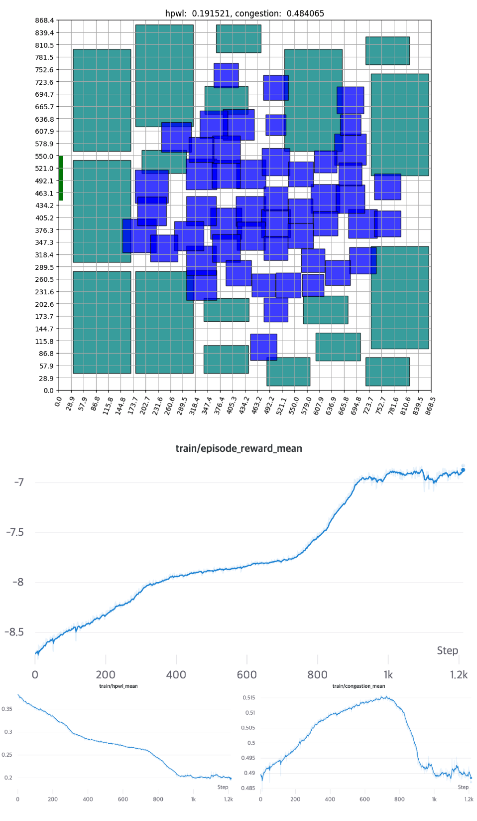
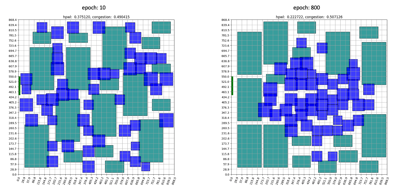
placment at 10 epochs and 800 epochs — [Figure ] - Placement result at 10 epochs and placement result at 800 epochs

The components that were placed randomly at the start of the training reveal that, as the training progresses, the standard cell is positioned in the center and the macro is on the outside. This configuration closely resembles expert placement or auto placement using tools. The training graph shows that the initial priority lies in minimizing the intuitive HPWL before moving on to fine-grained position exchange and congestion reduction. HPWL, which primarily focuses on ‘closely located components,’ experiences a rapid reduction right from the start of the learning process. In contrast, it is evident that HPWL has a more significant impact on learning at the beginning, as the congestion value increases at the start. It converges after approximately 1000 epochs if no additional heuristics are used.

How good is this result?

The preceding results, in fact, merely illustrate the agent’s learning process, not its capability. To confirm that the learning outcomes are genuinely acceptable, the exact data must be measured using an EDA tool, such as ICC2. The results of the simulation are presented in the table below.

WNS: Worst Negative Slack
FREQ: Frequency

Path Group	Human Experts		ICC2		Single Cluster		Bouding Box		Vanilla RL
Path Group	WNS	FREQ (MHz)	WNS	FREQ (MHz)	WNS	FREQ (MHz)	WNS	FREQ (MHz)	WNS	FREQ (MHz)
Group 0	0.00	143	0.00	143	0.00	143	0.00	143	0.00	143
Group 1	0.05	143	0.06	144	0.14	146	0.05	144	0.07	144
Group 2	0.45	153	0.42	152	0.49	154	0.43	152	0.42	152
Group 3	0.79	161	0.79	161	0.65	158	0.69	158	0.79	160
Group 4	2.60	227	2.65	230	2.66	230	2.60	227	2.55	230
Group 5	2.67	231	2.74	235	2.73	234	2.68	231	2.63	234

WNS and FREQ are the most essential figures for the floorplan. The disparity between the actual arrival time and the expected time of the design when the signal is transmitted to each component is referred to as WNS. If it is less than zero, it is considered a violation of the designed condition, and floorplan must be repeated. FREQ, on the other hand, measures the number of signals that can be processed per second, or operation speed. As a result, it is important whether WNS is positive, and how high FREQ is. Each group is a predetermined set of routing paths for performance testing. Therefore, ‘Performance is good when WNS is more than zero for each group and FREQ is high.’ (Please see ASIC-Chip-Placement Part 1 for a complete description of each indicator.) Take a look at the results; our agent displays statistics that are very close to the two baselines.

What problems need to be solved in the future?

The MakinaRocks COP team’s reinforcement learning-based algorithm has produced impressive learning outcomes for a relatively small netlist of approximately 120,000 standard cells. Based on this, our intention is to scale up to larger netlists and, ultimately, to leverage generalization as a tool for addressing various problems. However, to achieve this goal, there are still challenges that must be addressed in the future.

How can we achieve better placement outcomes with reducing learning time?
How can we attain good outcomes with minimal learning time for netlists that we haven’t seen after learning about multiple netlists?

To tackle the aforementioned challenges, our team is exploring the application of various optimization techniques, including simulated annealing, genetic algorithm, and force-directed method, as well as reinforcement learning. Furthermore, we plan to deploy 1 million units of components, which is the actual scale used in the field. Ultimately, our aim is to develop a product that can more effectively address the semiconductor floorplan challenge than current methods.

APPENDIX

Techniques for dealing with various challenges encountered during the project are introduced.

A. Action Design

A.1. Grid Cell Size Decision

When designing actions, keep the search field as small as possible while maximizing rewards. The size of the grid cell is critical from this perspective. If the grid cell is too small, it may be able to search in sufficient depth, but training time and complexity will grow exponentially. In contrast, if the grid cell is too large, the agent will be unable to execute fine-grained navigation. Furthermore, when components are randomly organized according to the size of the grid cell, space limitations often prevent the arrangement of all components. As a result, we proceeded to arrange each number of grid cell sizes in a given range at random and established the size of the grid cell with a high likelihood of inserting all components.

A.2. Invalid Action Masking

The area in which the next component can be placed varies depending on the present placement. To begin with, regardless of component type, it must not extend beyond the chip canvas. In the case of macro, there should be no overlap with other components, and in the case of standard cell, placement should consider the available area and density. Invalid action masking is the operation to successfully control the action based on these criteria. This is illustrated in the figure below.

B. Reward Function Design

B.1. Normalization & Reward Coefficient

To appropriately adjust the wire length and congestion set above, normalization and coefficient must be used. First, normalization is used to place two values within a specific range.

Wire Length

When the two net components are diagonally opposite each other on the chip canvas, HPWL reaches its maximum value. After computing HPWL for each net, divide it by the maximum value to effectively bound to a value between [0, 1].

Congestion

Dealing with congestion is slightly more complex than wire length. There are four sorts of edges formed by the minimum spanning tree or the steiner tree that travel through a specific grid cell.

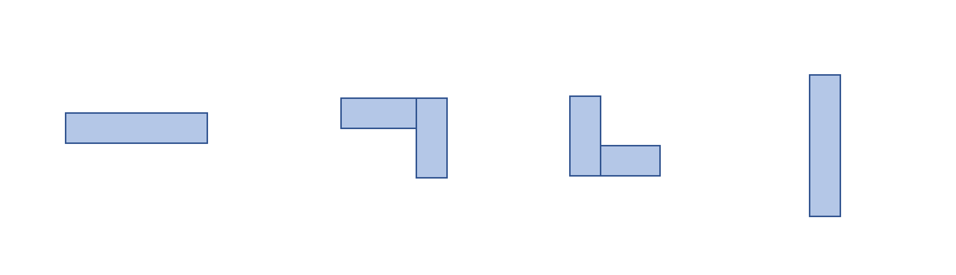
4 paths of edge — [Figure ] - 4 types of Edge passing through Grid Cell

It can be seen that the average value of horizontal and vertical congestion for all four categories yields 0.5. In other words, in the worst-case scenario, all of a net’s edges can be conceived of as passing through a single grid cell. Given this, if the congestion value is 0.5 X n_edges in this scenario, bounding can be achieved within the range of [0, 1], when the congestion for each net is split by the corresponding value.

Scaling is conducted between the two after normalization for wire length and congestion, respectively, by multiplying the coefficient.

\[R_{p,g}=-\alpha \cdot WireLength(p,g) - \beta \cdot Congestion(p,g) \qquad \text{s.t. } \text{density}(p,g) \leq \text{max}_\text{density}\]

B.2. Invalid Episode Handling

When placing components, there are times when all grid cells are placed in an unplaceable state before the rest of the components are. Overlapping is not allowed in macro, and this issue arises due to a lack of space for large macro components. Sorting the items by size can reduce the likelihood of this occurrence. However, simply sorting the placement isn’t a complete solution; the agent must be advised that the worst-case scenario is that the placement cannot be done. When an invalid episode occurs, the environment returns a value, which is the reward’s lower bound $-\alpha-\beta$. To improve the total value of the incentives, the agent learns that invalid episodes should not occur.

B.3. Convolution Filter

Clustering is initially performed to facilitate the calculation of tens of millions of standard cells. This leads to a large number of components being associated with a single cluster, resulting in an exceedingly high congestion value at that point. In light of this, the convolution filter is used to alleviate the resultant congestion map.

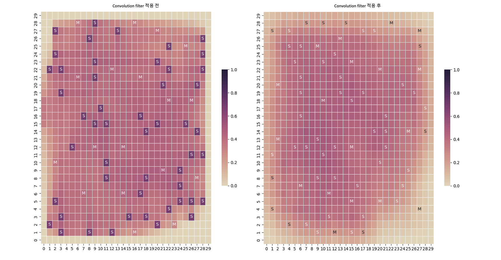
The congestion that are unduly concentrated on the standard cell cluster (grid cell indicated with S in the figure) are efficiently alleviated, as shown in the figure above. By extending congestion to the adjacent area, this procedure also reduces inaccuracies in the original data generated by clustering.

References

[1] Azalia Mirhoseini, Anna Goldie, Mustafa Yazgan, Joe Jiang, Ebrahim Songhori, Shen Wang, Young-Joon Lee, Eric Johnson, Omkar Pathak, Sungmin Bae, Azade Nazi, Jiwoo Pak, Andy Tong, Kavya Srinivasa, William Hang, Emre Tuncer, Anand Babu, Quoc V. Le, James Laudon, Richard Ho, Roger Carpenter, Jeff Dean, 2021, A graph placement methodology for fast chip design.
[2] Google AI, 2020, Chip Placement with Deep Reinforcement Learning, Google AI Blog.
[3] S. Kirkpatrick, C. D. Gelatt, Jr., M. P. Vecchi, 1983, Optimization by Simulated Annealing.
[4] Henrik Esbensen, 1992, A Genetic Algorithm for Macro Cell Placement.
[5] George E. Monahan, 1982, State of the Art—A Survey of Partially Observable Markov Decision Processes: Theory, Models, and Algorithms.
[6] G. Karypis, R. Aggarwal, V. Kumar, S. Shekhar, 1999, IMultilevel hypergraph partitioning: applications in VLSI domain.
[7] An Introduction to Routing Congestion, 2007, In: Routing Congestion in VLSI Circuits: Estimation and Optimization. Series on Integrated Circuits and Systems.
[8] Irwan Bello, Hieu Pham, Quoc V. Le, Mohammad Norouzi, Samy Bengio, 2016, Neural Combinatorial Optimization with Reinforcement Learning.
[9] Hanjun Dai, Elias B. Khalil, Yuyu Zhang, Bistra Dilkina, Le Song, 2017, Learning Combinatorial Optimization Algorithms over Graphs.